Control of a Batch
Process |
1) Signals, Systems and Control Department
Faculty of Mathematical Sciences
University of Twente
The Netherlands
2) Kodak Corporation
| To download the application in .pdf format, click here. |
Introduction
However, there frequently are more outputs than ”control knobs” to use for adjustment, and the inputs frequently affect many outputs simultaneously. Testing delay, more outputs than inputs, the desire for a first-order return rather than a step return to target for some products, and stochastic disturbances make this an interesting control problem.
Below is the transfer function plus disturbance model for a process like the one described above.

Here
The three outputs
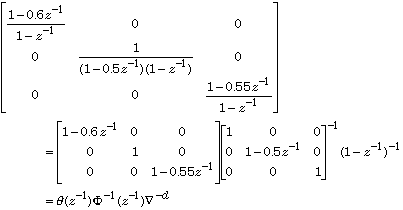
The three disturbance models are first order integrated moving average, first order integrated autoregressive, and first order integrated moving average, respectively.
Design TargetsThe control law H for this problem follows by the minimization of a mean square error criterion of the form
![]()
E denotes the expectation, e(t) is the deviation of the output y(t) from its set point, and

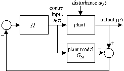
Fig. 1. Internal Model Control
Process
& Disturbance Models
The control is computed by a polynomial algorithm. To this
end, the plant-disturbance model is rendered as
![]()
with D(t) the effect of the disturbances on the output y. The process model
![]()
with L and R polynomial matrices in the delay operator
![]()
with v a column vector of white noise inputs. The quantities
![]()
![]()
for the plant. The polynomial matrix
![]()
The superscript * denotes the adjoint, that is,
![]()
The spectral factor
The controller H may now be expressed as
![]()
where the polynomial matrix T, together with the polynomial matrix P, is the solution of the two-sided equation
![]()

reveals that

Furthermore, writing

we see that

The weighting matrices, finally, are selected as

% demoB
% Script for the demo "Control of a batch process"
% Define the data
L = [-77*z^-3 0.33*z^-3; 0 0.03*z^-3; 0 0.1*z^-3];
R = eye(2,2);
theta = diag([1-0.6*z^-1 1 1-0.55*z^-1]);
Phi = diag([1 1-0.5*z^-1 1]);
d = 1;
Q1 = diag([0.01 8 2.25]);
Nabla = (1-z^-1);
% Spectral factorization
Gamma = spf(L'*Q1*L);
The result is
Gamma
Constant polynomial matrix: 2-by-2
Gamma =
7.7 -0.033
0.00074 0.17
![]()
for the matrices T and P. For this we use the routine
axybc. This solves the two-sided polynomial matrix equation![]()
To turn into a polynomial matrix equation we need to multiply it by a suitable power n of
Choosing n = 3 we have
% Solution of the two-sided
equation
n = 3;
A = z^-n*Gamma';
B = Nabla^d*Phi;
C = L'*Q1*theta;
[T,U] = axybc(A,B,C);
T turns out to be 2×3 matrix of degree 1, as predicted by the theory (MacGregor and Harris, 1987):
T =
-0.04 -0.00025 + 0.00012z^-1
-5.6e-005
-3.8e-006 2.6 - 1.2z^-1 0.59
![]()
where
![]()
is polynomial because
% Compute the controller H =
phi/theta
phi = R/Gamma*T;
The result is
phi =
-0.0052 0.065 - 0.03z^-1 0.015
-1.3e-016 15 - 7.1z^-1 3.4
![]()
The closed-loop response to the disturbances D(t) follows from the sensitivity matrix S:

It is not difficult to find from the block diagram of Fig. 1 that if the plant model exactly matches the plant then
![]()
It follows that

where
![]()
Thus we add the lines
% Compute the sensitivity
matrix S = psi/theta
psi = theta-L/Gamma*T;
% Plot the data
figure; clf
k = length(r);
for i = 1:k
for j = 1:k
subplot(k,k,(i-1)*k+j)
plot(0:n,r{:}(i,j))
grid on; axis([0 n -1.5 1.5])
end
end
Matlab produces the plot of Fig. 2 for the impulse response matrix. The step responses may be computed similarly and are shown in Fig. 3.
% Compute and plot the
disturbance step response matrix s
% Apply long division to (psi/theta)*1/(1-z^-1)
n = 10;
[q,s] = longrdiv(psi,theta*(1-z^-1),n);
% Plot
figure; clf
k = length(s);
for i = 1:k
for j = 1:k
subplot(k,k,(i-1)*k+j)
plot(0:n,s{:}(i,j))
grid on; axis([0 n -1.5 1.5])
end
end
Fig. 3. Disturbance step response matrix
Assesment