Applications in Behavioral Theory
 

Huibert Kwakernaak

Signals, Systems and Control Department
Faculty of Mathematical Sciences
University of Twente
The Netherlands

To download the application in .pdf format, click here.


Introduction
Example 1
Kernel Representation
Full and Manifest Behavior
Example 2
Controlability

Image Representation
State Representation
Example 3

IO System Construction
Example 4

Introduction
Behavioral system theory (Polderman and Willems, 1998) is a very general approach to system theory. It defines a system as a relation between the signals that constitute the environment of the system. A distinction is made between latent (or internal) and manifest (or external) signals but not necessarily between input and output signals.

Polynomial matrices play an important role in the behavioral theory of linear systems. The purpose of this demo is to show that the Polynomial Toolbox provides many useful routines for dealing with problems and questions in behavioral linear system theory.
polyx: the polynomial toolbox 2.0

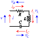
Fig. 1. RCL network

Example
By way of illustration we consider the simple electrical network of Fig. 1. The signals of interest are the currents polynomials, polynomial equations and polynomial matrices through the resistor, inductor and capacitor, respectively, the voltages control systems analysis, signal processing and across these same network elements, the current that flows into the network, and the voltage control systems analysis across the network. The relations between the signals are given by

resistor:

inductor:

capacitor:

All these equations can be combined in the form

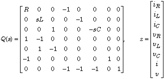
where the polynomial matrix Q and the vector-valued signal z are given by
numerical algorithm

Kernel Representation
The representation is called a kernel representation of the system, because it defines the system as all signals that are in the kernel (or null space) of the operator .

Full & Manifest Behavior
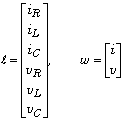
The equation (5) characterizes what is known as the full behavior of the system, because it includes all latent and manifest signals. Such a characterization is typically obtained when setting up the system equations from first principles. For the electrical network the latent variables and the manifest variables w could be chosen as

If the latent variables are eliminated from the behavior then the manifest behavior is obtained.

Compensation of the Manifest Behavior
We consider how to compute the manifest behavior from the full behavior. Partitioning the matrix Q as we have for the full behavior

where s represents the differentiation operator. Let the rows of the polynomial matrix be a minimal polynomial basis for the left null space of . Then the manifest behavior has the kernel representation

where

Example
In the example, choose the numerical values

We input the polynomial matrix Q as

R = 3; L = 1; C = 1/2;

Q = [ R 0 0 -1 0 0 0 0
0 s*L 0 0 -1 0 0 0
0 0 1 0 0 -s*C 0 0
1 -1 0 0 0 0 0 0
0 1 -1 0 0 0 0 0
-1 0 0 0 0 0 1 0
0 0 0 -1 -1 -1 0 1];

The polynomial matrices and follow as

Q1 = Q(:,1:6); Q2 = Q(:,7:8);

From this, the matrices and may be computed as

N = null(Q1')'; R = N*Q2

R =
2 + 3s + s^2 -s

Hence, the manifest behavior is described by the differential equation

Controllability
A behavioral system in kernel representation is controllable iff the polynomial matrix R is left prime (Polderman and Willems, 1998). For the example we can easily verify controllability by typing

isprime(R)

ans =
1

images/demo_behav/Image Representation
A well-known fact from behavioral theory is that given a controllable kernel representation

there always exists an equivalent images/demo_behav/Image representation of the form

with a latent variable. Inspection shows that the columns of need to be a minimal basis for the right null space of . Thus, for the example we may compute M as

M = null(R)

M =
s
2 + 3s + s^2

Hence, the images/demo_behav/Image representation of the system is

Note that physically the latent variable corresponds to , which happens to be the charge of the capacitor.

State Representation
Another fact from behavioral system theory is that the manifest behavior of any finite-dimensional linear system may be represented in the equivalent state space form

The latent variable x is the state of the system. This representation is by no means unique, and may be constructed in the following way from the kernel representation .

First, assume that R is row-reduced. If it is not then it may be unimodularly transformed to be row-reduced without changing the behavior.

Let S be a square, nonsingular, row-reduced matrix whose row degrees equal the row degrees of R, and chosen such that is left coprime. Obviously the behavior is equivalent to the behavior defined by

Let

be a minimal realization of the left coprime matrix fraction . Then clearly

is a state realization of the behavior.

Example
We further pursue the example. Given the row-reduced polynomial matrix

R

R =
2 + 3s + s^2 -s

we choose

S = s^2;

A minimal realization of is obtained as

[A,B,C,D] = lmf2ss(R,S)

A =
0 1
0 0

B =
3.0000 -1.0000
2.0000 0

C =
1 0

D =
1 0

Construction of IO System
So far no distinction has been made among the manifest variable between ”input” and ”output” variables, which the obvious connotation of ”causes” for inputs and ”effects” for outputs. Indeed, in the electrical network example there is no a priori reason which of the two manifest variables v and i is the input and which is the output because the circuit could be connected to a voltage or a to a current source.

If no compelling reason exists to designate certain manifest variables as inputs and other variables as outputs then possible partitionings of the manifest variables into sets of input variables and output variables may be determined on the basis of the (plausible) requirement that the outputs are causally affected by the inputs.

To make this more concrete, suppose that we have a kernel representation such that R has full row rank with rank equal to r. Select r components of w as outputs and permute the components of w and the corresponding columns of R such that the selected outputs are the first r components of w. We write the resulting kernel representation as

with y the output and u the input. Then the proposed selection of outputs and inputs is deemed acceptable if is proper.

Consider the state representation

where C and D have r rows. Then in this context a causal IO representation may be constructed by selecting r columns of D so that the resulting square submatrix is nonsingular. By designating the corresponding entries of w as outputs and the remaining entries as inputs the equation may be rearranged as . Substitution of y into the equation results in a state representation of the IO system.
Example
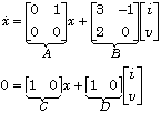
We found that the electrical network has the state representation

Inspection of the matrix D shows that the only available option is to take the current i as the output and, hence, the voltage as the input. Substitution of the resulting output

into the first equation yields the corresponding state differential equation. Not wanting to make any mistakes we invoke Matlab:

c = [-1 0]; B1 = B(:,1); B2 = B(:,2);
a = A+B1*c, b = B2

a =
-3.0000 1.0000
-2.0000 0

b =
-1.0000
0

Thus, we have the IO representation

This selection of input and output corresponds to connecting the network to a voltage source. Connecting it to a current source does not lead to a causal IO system because the admittance

of the network is nonproper.