Mixed Sensitivity Demo

Polynomial Solution of the SISO Mixed Sensitivity H-infinity Problem

Signals, Systems and Control Department
Faculty of Mathematical Sciences
University of Twente
The Netherlands

To download the application in .pdf format, click here.

Synopsis
Introduction
Example 1: Scalar Process
LMF Representation
Frequency Domain Solution
Spectral Factorization
The Compensator
Closed Loop Poles

Approaching the Optimal Solution
Optimal Compensator
Assessment of the Design
Alternative Spectral Factorization
Automating the Search
Zero-pole Cancelation
The Function MIXEDS

Synopsis
Mixed sensitivity optimization is a powerful design tool for linear single-degree-of-freedom feedback systems. It allows simultaneous design for performance and robustness, and relies on shaping the two critical closed-loop sensitivity functions with frequency dependent weights.

To obtain satisfactory high-frequency roll-off nonproper weighting functions may be needed. These cannot be directly handled in the conventional state space solution of the H-infinity problem. Nonproper weighting functions present no problems in the frequency domain solution of the H-infinity problem. The frequency domain solution may be implemented in terms of polynomial matrix manipulations.

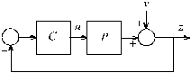
We present the mixed sensitivity problem and its solution for single-input-single-output plants. Step by step the Toolbox function mixeds is developed that implements the algorithm. A simple but relevant example is used for illustration.

Introduction
To demonstrate the capabilities of the Polynomial Toolbox we implement the polynomial solution of a mixed sensitivity H-infinity problem. Consider the single-degree-of-freedom feedback loop of Fig. 1. P is the plant transfer matrix and C the compensator transfer matrix.

polynomial equations

Fig. 1. Single-degree-of-freedom feedback loop

The sensitivity matrix S and input sensitivity matrix U of the feedback system are defined as

The mixed sensitivity problem is the problem of minimizing the infinity norm of

with suitably chosen weighting matrices and , and V a suitably chosen shaping matrix. In the SISO case the infinity norm is given by

The problem may be reduced to a ”standard” H-infinity problem by considering the block diagram of Fig. 2, which includes the weighting and shaping filters.

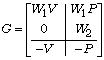
The diagram of Fig. 2 defines a standard problem whose ”generalized plant” has the transfer matrix

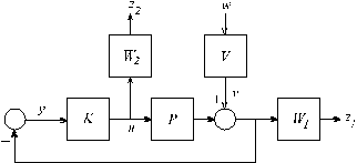
Fig. 2. Mixed sensitivity configuration

The closed-loop transfer matrix from w to

is precisely the function H whose infinity-norm we wish to minimize.

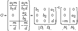
There are many ways to solve this problem, but only the frequency domain solution (Kwakernaak, 1996) allows the generalized plant to have a nonproper transfer matrix G. To enhance robustness at high frequencies it usually is necessary to make the weighting filter nonproper, which in turn makes G nonproper.

For simplicity we develop the solution for the SISO case only. Suppose that

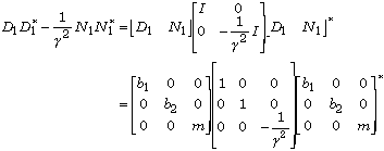
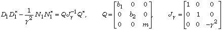
where the numerators and denominators are (scalar) polynomials. Note that P and V have the same denominators d — this makes partial pole placement possible (Kwakernaak, 1993).

Numerical Example
We study in particular the following numerical example (Kwakernaak, 1963):

where we let c = r = 1. Note that is nonproper and, hence, the generalized plant G is nonproper. The various polynomials are defined by the following command lines:

% Define the data
n = 1; d = s^2; m = s^2+s*sqrt(2)+1;
c = 1; r = 1; a1 = 1; b1 = 1; a2 = c*(1+r*s); b2 = 1;

LMF Coprime Factorization
The frequency domain solution of the problem of Kwakernaak (1996) is based on polynomial matrix manipulations. It requires G to be represented in left coprime polynomial matrix fraction form. The desired left coprime factorization is

The partitioning is needed for the solution of the problem. The following code lines define the various polynomial matrices:

% Define the various polynomial matrices
D1 = [b1 0; 0 b2; 0 0];
D2 = [a1 ; 0 ; d ];
N1 = [ 0; 0; -m ];
N2 = [ 0; a2; -n ];

These code lines are actually taken from the macro mixeds, which automates the entire computation.

Frequency Domain Solution of the H-infinity Problem
As usual in the solution of the problem we consider the problem of finding a compensator that stabilizes the system and makes the infinity norm of the closed-loop transfer matrix less than or equal to a given number . Define the rational matrix

The * denotes conjugation, that is, . In the next subsection it is seen how a spectral factorization

of may be obtained. The spectral factor is a square rational matrix such that both and have all their poles in the open left-half plane. The matrix J is a signature matrix of the form

where the two unit matrices do not necessarily have the same dimensions.

Given this spectral factorization, all compensators whose norm is less than the number are of the form , where

U is a rational stable matrix such that . In particular one may chose .

Spectral Factorization
We consider the spectral factorization

It requires the following steps.

Do the polynomial spectral cofactorization

Perform the ”left-to-right” conversion

Do the polynomial factorization

Then the desired spectral factor is

The first spectral factorization may actually be done analytically, because we have

Inspection shows that if each of the polynomials , and is strictly Hurwitz then the desired spectral factorization may be rendered in slightly modified form as

The computation of the left-to-right conversion

may easily be coded.

% Left-to-right conversion
Q = diag([b1 b2 m]);
[Del,Lam] = lmf2rmf([N2 D2],Q)

The result is

Del =

-0.71 0.71 + s
0.71 + 1.7s + s^2 0.71 + 0.71s
-0.71 -0.71 + s

Lam =

0.71 + s 0.71
-0.71 0.71 + s

The second spectral factorization now takes the form

It is not difficult to write the necessary code lines

% Define gamma
gamma = 4;

% Spectral factorization
Jgamma = eye(3); Jgamma(3,3)= -gamma^2;
DelDel = Del'*Jgamma*Del;
[Gam,J] = spf(DelDel)

Gam =

-1.3e+002 - 50s - s^2 -2.2e+002 - 0.046s
1.3e+002 + 48s + 0.17s^2 2.2e+002 - 3.8s

J =

1 0
0 -1

Computation of the Compensator
To determine the numerator Y and denominator X of the compensator we need to compute

where for simplicity we choose . It is advantageous to implement this computation as a right-to-left conversion

so that the compensator transfer function is

Again this may be coded straightforwardly:

% Computation of the compensator
xy = rmf2lmf([1 0]*Gam,Lam);
x = xy(1,1), y = xy(1,2)

The output is

x =

2.4e+002 + 1.6e+002s + 50s^2 + s^3

y =

63 + 1.8e+002s - 0.66s^2

Computation of the Closed Loop Poles
The closed-loop characteristic polynomial is

We use it to test closed-loop stability and to compute the closed-loop poles.

% Computation of the closed-loop characteristic polynomial
% and closed-loop poles
phi = d*x+n*y;
clpoles = roots(phi)

clpoles =
-46.7980
-0.9727 + 0.6271i
-0.9727 - 0.6271i
-0.7071 + 0.7071i
-0.7071 - 0.7071i

Approaching the Optimal Solution
It is easy to collect the command lines listed so far in an m-script and to run the script repeatedly for different values of .

We first run the script with gamma = 4. The closed-loop poles all have negative real parts, and, hence, the closed-loop system is stable.

Next, we run the macro with gamma = 3.5. The script returns

clpoles =

4.9995
-0.9590 + 0.5600i
-0.9590 - 0.5600i
-0.7071 + 0.7071i
-0.7071 - 0.7071i

The closed-loop system is unstable. Hence, gamma has been chosen too small.

Note that four of the five closed-loop poles do not change much with gamma. The fifth pole is very sensitive to changes in gamma.

We test this dependence by running the script several times for different values of gamma without showing the output. Table 1 shows the results. Apparently as gamma decreases the fifth pole crosses over from the left- to the right-half complex plane, but does so through infinity.

For the final run we take gamma = 3.9515, close to the optimal value but such that the closed-loop system is stable. The corresponding numerator polynomial y and the denominator polynomial x of the compensator are

y =
4e+003 + 1.1e+004s - 0.66s^2

x =
1.5e+004 + 1e+004s + 3e+003s^2 + s^3

Table 1. Dependence of the fifth pole on gamma

gamma	the fifth pole
4	–46.798
3.5	4.9995
3.75	11.369
3.875	30.297
3.9375	173.86
3.9688	–127.80
3.95	315.38
3.951	3153.8
3.9515	–2987.6

Optimal Compensator Calculation
Inspection of the numerator and denominator polynomials y and x of the compensator obtained for gamma = 3.9515 shows that their coefficients are large, except for the leading coefficients.

In fact, we may cancel the leading coefficients and simplify y and x. This amounts to cancelling the compensator pole-zero pair and eliminating the corresponding closed-loop pole that pass through infinity as gamma passes through the optimal value.

Recalculation of the closed-loop poles after this cancellation confirms that the large closed-loop pole has disappeared. These calculations are performed by typing a few simple command lines

y{2} = 0; x{3} = 0;
y = y/x{2}, x = x/x{2}

y =
1.3 + 3.8s

x =
5.1 + 3.4s + s^2

phi = d*x+n*y;
clpoles = roots(phi)

clpoles =
-0.9703 + 0.6201i
-0.9703 - 0.6201i
-0.7075 + 0.7072i
-0.7075 - 0.7072i

Assessment of the Design
To assess the design we calculate and plot the sensitivity function S and the complementary sensitivity function T of the closed-loop system. They are given by

We type in the command lines

omega = logspace(-2,2); j = sqrt(-1);
S = bode(pol2mat(d*x),pol2mat(phi),omega);
T = bode(pol2mat(n*y),pol2mat(phi),omega);
figure(1);
loglog(omega,abs(S),'k'); hold on
loglog(omega,abs(T),'b'); grid on
text(.1,.01,'S'), text(10,.01,'T')

Fig. 3 shows the plots of S and T. For a discussion of the design and the mixed sensitivity design methodology see Kwakernaak (1993).

Alternative Spectral Factorization
As we have seen, the spectral factorization behaves poorly as the optimal solution is approached. The reason is that the factorization becomes ”noncanonical” (Kwakernaak, 1996). This difficulty may be remedied by using an alternative form for the second polynomial spectral factorization. Instead of factoring

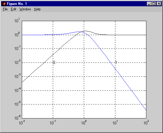
Fig. 3. Magnitude plots of the sensitivity functions

we rearrange the factorization as

L is diagonal in the form

where and are diagonal nonnegative-definite but not unit matrices. If the factorization is close to noncanonical then L is close to nonsingular. The large numbers disappear.

The alternative factorization is obtained by an option in the spf command. The computation of the compensator is not affected, so we only need to change the code line that contains the spf command to

[Gam,J] = spf(DelDel,'nnc');

Rerunning the script with this modification for gamma = 3.9515 shows that the large numbers have disappeared. We also see that instead of the large closed-loop poles and corresponding large pole and zero of the compensator we now have a closed-loop pole, compensator pole and zero at –1:

y,x

y =
1.3 + 5.1s + 3.8s^2

x =
5.1 + 8.4s + 4.4s^2 + s^3

rootsx = roots(x), rootsy = roots(y), clpoles

rootsx =
-1.6787 + 1.5027i
-1.6787 - 1.5027i
-1.0000

rootsy =
-1.0000
-0.3476

clpoles =
-0.7071 + 0.7071i
-0.7071 - 0.7071i
-1.0002
-0.9715 + 0.6197i
-0.9715 - 0.6197i

Cancellation of the common root of y and x leads to the same optimal compensator that was previously obtained:

x/(s-rootsx(3)), y/(s-rootsy(1))

ans =
5.1 + 3.4s + s^2

ans =
1.3 + 3.8s

Automating the Search
Now that the numerical instability in the computation of the compensator has been removed it is simple to automate the search process. We implement a binary search that involves the following steps:

Specify a minimal value gmin and a maximal value gmax for gamma.

Test if a stabilizing compensator is found at gamma = gmax. If not then stop.

Test if a stabilizing compensator is found at gamma = gmin. If yes then stop.

Let gamma = (gmin+gmax)/2. If a stabilizing compensator is found then let gmax = gamma, otherwise let gmin = gamma.

If gmax-gmin is greater than a prespecified accuracy then return to 4.

Retain the solution for gamma = gmax and stop.

This search algorithm has been implemented in the macro mixeds. Calling the routine in the form

gmin = 3.5; gmax = 4; accuracy = 1e-4;
[y,x,gopt] = mixeds(n,m,d,a1,b1,a2,b2,gmin,gmax,accuracy,'show')

executes the search while showing the intermediate results. The search stops if gmax-gmin is less than the input parameter accuracy. This is the output:

gamma test result
----- -----------
4 stable
3.5 unstable
3.75 unstable
3.875 unstable
3.9375 unstable
3.96875 stable
3.95313 stable
3.94531 unstable
3.94922 unstable
3.95117 stable
3.9502 unstable
3.95068 unstable
3.95093 stable
3.95081 stable
3.95074 stable

Cancel root at -0.999999

y =
1.3 + 3.8s

x =
5.1 + 3.4s + s^2

gopt =
3.9507

Cancelling pole-zero pairs
The numerator x and the denominator y of the optimal compensator turn out to have a common root. This often happens. The precise location of this spurious pole-zero pair is unpredictable. It needs to be cancelled in the compensator transfer function .

Rather than relying on one of the polynomial division routines we write a few dedicated code lines. Suppose that the numerator y has a root z. Then by polynomial division we have for the denominator x

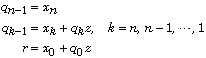
where the remainder r is a constant. By substituting s = z we see that actually r = x(z). Expanding the polynomials x and q as

it follows that the quotient q and the remainder r may recursively be computed as

Note that this way of computing r = x(z) is nothing else than Horner's algorithm. If the remainder r is small then we cancel the factor s–z. By the same algorithm the factor s–z may be cancelled from the numerator y.

These are the necessary code lines. A tolerance tolcncl is used to test if the remainder is small.

% Cancel any common roots of xopt and yopt
rootsy = roots(yopt);
xo = xopt{:}; degxo = deg(xopt);
yo = yopt{:}; degyo = deg(yopt);
for i = 1:length(rootsy)
z = rootsy(i);

% Divide xo(s) by s-z
q = zeros(1,degxo);
q(degxo) = xo(degxo+1);
for j = degxo-1:-1:1
q(j) = xo(j+1)+z*q(j+1);
end

% If the remainder is small then cancel
% the factor s-z both in xo and in yo
if abs(xo(1)+z*q(1)) < tolcncl*norm(xo,1)
xo = q; degxo = degxo-1;
p = zeros(1,degyo);
p(degyo) = yo(degyo+1);
for j = degyo-1:-1:1
p(j) = yo(j+1)+z*p(j+1);
end
yo = p; degyo = degyo-1;
if show
disp(sprintf('\nCancel root at %g\n',z));
end
end
end

The Function MIXEDS
The full command

[y,x,gopt] = ...
mixeds(n,m,d,a1,b1,a2,b2,gmin,gmax,accuracy,tol,'show')

includes a four-dimensional optional tolerance parameter

tol = [tolcncl tolstable tolspf tollr]

which allows to fine tune the macro. For a description of the various tolerances consult the manual page for mixeds.