Achievable
Feedback Performance |
Signals, Systems and Control
Department
Faculty of Mathematical Sciences
University of Twente
The Netherlands
| To download the application in .pdf format (97 k), click here. |
| Introduction SISO minimal peak values SISO computation of the minimum |
The macro minsens MIMO minimal peak values MIMO example |
Introduction
![]()
and complementary sensitivity matrix
![]()
These properties include the sensitivity of the feedback loop to disturbances and measurement noise, its response to reference inputs, and its stability and performance robustness (Kwakernaak, 1995).
![]()
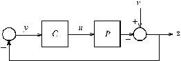
Fig. 1. LTI feedback system
Especially for complex design problems it is highly recommended to devote some time to exploratory analysis before attempting the actual design. This exploratory analysis serves to reveal the inherent possibilities and limitations of the control system. Part of this exploratory analysis always is the computation of the poles and zeros of the plant. Any right-half plane zeros and poles that are present impose essential constraints on the closed-loop bandwidth that may be achieved or is necessary (again see Kwakernaak, 1995, for a review).
For MIMO systems the open-loop pole and zero locations do not fully reveal the design limitations. For instance, in the SISO case the presence of a nearly cancelling pole-zero pair in the right-half plane predicts poor performance, with high peaks in the sensitivity functions. The closer the pole and zero are, the higher the peak. In the case of MIMO systems the pole of such a pair may occur in a different ”channel” than the zero so that the pole and zero do not interact and their adverse effects are not amplified such as in the SISO case.
To reveal the a priori design limitations more fully it may be useful to compute the minimal peak values of the
SISO minimal peak values for the sensitivities
![]()
The polynomial N is the plant numerator polynomial and the polynomial D is the plant denominator polynomial.
The minimal peak value of the
![]()
for the scalar
![]()
If the plant is strictly proper then
![]()
![]()
The properties of the minimum peak value may be summarized as follows:
.
For the minimal peak value of the complementary sensitivity function T similar results hold. The critical equation that needs to be solved now is
![]()
and the optimal complementary function is
![]()
This is the summary of the results for the minimization of
.
SISO computation of the minimum
peak value
The only situation where some serious
computation needs to be done once the open-loop poles and zeros are available arises when
the plant has both right half plane zeros and poles. We then need to solve the polynomial
equation
![]()
The solution of this problem provides the minimal peak value of both the sensitivity and the complementary sensitivity function. If
![]()
and introduce the column vectors
Then it may be verified that the polynomial equation we need to solve is equivalent to the matrix equation
![]()
![]()
![]()
To show that amounts to a generalized eigenvalue problem we rearrange it in the form
![]()
This is equivalent to the equation
![]()
where
We need the solution of that corresponds to the real eigenvalue
The macro minsens
We develop a new Polynomial Toolbox function
minsens that computes the minimal peak value of the sensitivity functions. Its input
arguments are the numerator polynomial N and the denominator polynomial D of
the SISO plant.
As we develop the macro we test it for the plant with transfer function
![]()
We input the data accordingly as
The first few lines of the m-file are
% minsens
% The function
% p = minsens(N,D)
% computes the minimum peak value of the sensitivity and
% complementary sensitivity functions for the SISO plant
% with transfer function P = N/D that may be achieved by
% feedback
function p = minsens(N,D)
This provides the help text, and declares the function, its input arguments and its output arguments.
Normally a sequence of tests needs to follow this preamble to check whether N and D are really scalar polynomials but we dispense with this for the purpose of this demo.
Given the numerator and denominator polynomials we now compute their roots and use these to define the polynomials
% Compute the polynomials Nplus and Dplus whose roots are
% the roots of N and D, respectively, with positive real parts
rootsN = roots(N); rootsNplus = rootsN(find(real(rootsN)>0));
Nplus = mat2pol(poly(rootsNplus));
rootsD = roots(D); rootsDplus = rootsD(find(real(rootsD)>0));
Dplus = mat2pol(poly(rootsDplus));
keyboard
The Matlab command poly is used to construct the polynomials Nplus and Dplus from their roots after which they are converted to Polynomial Toolbox format with the Toolbox command mat2pol. While developing the macro we end it with the keyboard command so that the results at that point may be inspected. In the present case typing the command
results in the output
K»
Editing this to
K» Nplus, Dplus
and ending the line with a return results in the output
Nplus =
-1 + s
We now include two tests to see whether the peak value is either 0 or 1.
% Check whether p = 0 or p = 1
if isempty(Nplus)
p = 0; return
elseif isempty(Dplus)
p = 1; return
end
For the example that we are pursuing both tests fail so we are in the situation where the generalized eigenvalue problem needs to be solved. We first set it up.
% Solve the generalized eigenvalue problem
A = [ sylv(Dplus,'col',n-1) sylv(Nplus,'col',d-1) ];
J = 1;
for i = 2:n
J(i,i) = -1*J(i-1,i-1);
end
B = [ sylv(Dplus','col',n-1)*J zeros(n+d,d) ];
Only one more line is needed to complete the macro:
p = 1/min(abs(eig(A,B)));
Calling
results for the example at hand in
We test a few more examples
minsens(s+1,s-1)
minsens(s-1,s+1)
minsens(s-1,s-1)
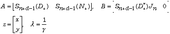
To bring the minimum sensitivity problem into standard form we consider the block diagram of Fig. 2. When the loop is opened the signals are related as
![]()
This defines the generalized plant of the standard problem as
![]()
If the plant P has the left coprime representation
![]()
After converting this left coprime fraction to descriptor form the routine dssrch may be called to solve the
D = prand([1;2],2,2,'int')
N = prand([1;2],2,2,'int')
The zeros and poles of the plant are
Zeros = roots(N)
Poles = roots(D)
Inspection shows that the plant has both right-half plane poles and zeros so by analogy to the SISO problem we expect a minimum peak sensitivity of at least 1.
We first convert the generalized plant into descriptor form:
Dg = [D zeros(2,2); eye(2,2)
eye(2,2)];
Ng = [D N; zeros(2,2) zeros(2,2)];
[A,B,C,D,E] = lmf2dss(Ng,Dg)
B =
0 0 85.0000 336.0000
0 0 -66.0000 -264.0000
0 0 -61.0000 -276.0000
C =
1 -6 0
0 -1 0
-1 6 0
0 1 0
D =
1.0000 0 11.0000 43.0000
0 1.0000 0 7.0000
-1.0000 0 -11.0000 -43.0000
0 -1.0000 0 -7.0000
E =
1 0 0
0 1 0
0 0 1
The solution of the
[Ak,Bk,Ck,Dk,Ek,gopt,clpoles] = dssrch(A,B,C,D,E,2,2,0.5,5)
The resulting output is
Bk =
-0.9241 -9.2055
1.7746 -0.6237
Ck =
0.0410 -0.0035
-0.1003 0.0981
Dk =
-0.3750 0.0976
0.0547 -0.0142
Ek =
1 0
0 1
gopt =
1.1595
clpoles =
-45.5167 + 0.0000i
-0.1755 - 0.9418i
-0.1755 + 0.9418i
-0.4833 - 0.0000i
-1.0000
We observe that the minimal norm is 1.1595. The fact that this number is not all that much greater than 1 indicates that a design without exaggerated peaking of the sensitivity functions is possible as long as the design specifications — in particular the desired bandwidth — are compatible with the limitations imposed by the right-half plane zeros and poles of the plant.