ARMA Process Demo

Computing the Covariance Matrix of an ARMA Process

Michael Sebek¹⁾, Huibert Kwakernaak²⁾

¹⁾Institute of Information Theory and Automation
Czech Academy of Sciences
The Czech Republic

²⁾Signals, Systems and Control Department
Faculty of Mathematical Sciences
University of Twente
The Netherlands

To download the application in .pdf format, click here.

Introduction
Algorithm
Example 1: Scalar Process

The Macro COVF
Example 2: Two-variable Process

Introduction
The problem of computing the covariance function for a given multivariable ARMA process is often encountered in estimation, filtering, stochastic control and communications.

Consider the ARMA process

where z is the shift operator defined by . A and B are square polynomial matrices in z with possibly complex-valued coefficients. The random sequence e is white noise so that

The superscript H indicates the complex conjugate transpose. A is assumed to be monic (that is, its leading coefficient matrix is nonsingular) with all its roots strictly inside the unit circle. Under these assumptions the ARMA process y is well-defined and asymptotically stationary.

The covariance matrix function that is to be found is defined by

Algorithm
The covariance matrix function may be computed by inverse z-transformation of the spectral density matrix

The computation of the covariance function (Söderström, Jezek and Kucera, 1997) follows by partial fraction expansion of the spectral density in the form

This partial fraction expansion is equivalent to solving the symmetric two-sided polynomial matrix equation

for the polynomial matrix X. Once X is available we may expand

polyx: the polynomial toolbox for matlab

by long polynomial division. Inspection of the right-hand side shows that

polynomial equations

Example 1: A Scalar Process
To illustrate the procedure first consider a scalar ARMA process y given by

We develop a Polynomial Toolbox function called covf, which takes the polynomial matrices A and C as input arguments and has the desired covariance function r as output. Because a macro with the same name exists in the System Identification Toolbox we need to overload this function. Practically this means that the macro is placed in the pol subdirectory of the main Polynomial Toolbox directory. When Matlab detects that covf is called with one or more polynomial objects as input argument then it uses the version of covf that is located in this subdirectory.

The Macro COVF
The first lines of the macro are

% covf
%
% This function computes the covariance function
% of the discrete-time ARMA process y defined by
%
% A(z)y(t) = C(z)e(t)
%
% with e standard white noise.

function r = covf(A,C,n)

The third input argument n is the number of time shifts over which the covariance function is required.

Normally at this point each Polynomial Toolbox function performs a number of correctness checks on the input arguments. We dispense with these for the purpose of this demo.

To solve the symmetric polynomial equation

we use the Toolbox function xaaxb. Only one line is needed:

% Solve the two-sided polynomial matrix equation
X = xaaxb(A,C*C');

For the example at hand the intermediate solution at this point is

X =
-20 + 8.3z + 28z^2

From the given polynomial A and the computed polynomial X the desired covariance function is recovered by "long division" of . For this purpose the macro longldiv is available. Given the square polynomial matrix D and the polynomial matrix N this function finds the first n + d + 1 terms of the Laurent series expansion

If the fraction is proper then the macro returns the first terms (with d an input parameter) of the expansion

This is exactly what we need. Thus, the appropriate command is

% Apply long division to X\A
[Q,R] = longldiv(X,A,n);

R is returned as a polynomial matrix in the variable of degree n. For convenience we also return the desired covariance function as a polynomial in this variable:

% Construct the covariance function
r = R;
r{0} = r{0}+r{0}';

The macro is now complete and we may apply it to the example:

r = covf(1-2.4*z+1.43*z^2,1,40);

The resulting covariance function r may be plotted using standard Matlab commands:

plot(0:40,r{:},'o')
title('Covariance function - Example 1')
xlabel('tau'), ylabel('r'), grid on

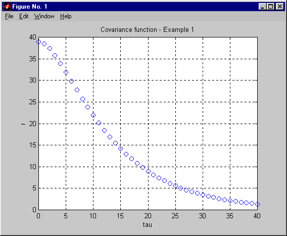
Fig. 1 shows the plot of the covariance function.

control engineers

Fig. 1. Covariance function of the ARMA process of Example 1

Example 2: Two-variable Process
As another example consider the computation of the covariance matrix function of the two-variable ARMA process y defined by

As our newly created function is ready for multivariable processes we may use it as it is after defining the data:

A = [1-2*z 0; 6 1-2.5*z]; C = eye(2,2);
r = covf(A,C,10);

The output r now is a polynomial matrix of degree 10. The coefficients r{i}, i = 1, 2, , 10, constitute the desired covariance function. They may be plotted in a single frame by the following sequence of standard Matlab commands that we include at the end of the macro covf:

% Plot the covariance function
figure; clf
k = length(C);

for i = 1:k
for j = 1:k
subplot(k,k,(i-1)*k+j)
plot(0:n,r{:}(i,j),'o')
grid on; xlabel('tau')
end
end

The resulting plot is shown in Fig. 2. The subplot in position (i, j) shows the scalar covariance function
.

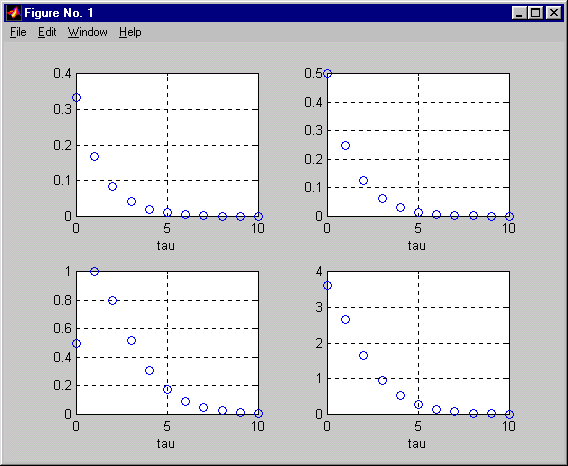
Fig. 2. Covariance function of the ARMA process of Example 2